Plotting (inverted) u-shapes in R

It seems that nowadays, no paper on optimal distinctiveness gets published without a graph on how the s-shaped mechanisms of legitimacy loss and competitive gain result in a curvilinear effect. I collected some information from countless threads and guides and provided a small tutorial on how to do this in R. Here you go:

First, we load the packages:

library(ggplot2) ## for plotting
library(truncnorm) ## for making truncated normal distributions
library(tikzDevice) ## for latex output
library(patchwork) ## to group plots

Then we create the logit function that helps us with the s-shapes.

## generate logit function for s-shape
f_logit <-function(b0,b1,b2,x) {
  1/(1+exp((b0 +b1*x+b2*(x^2))))
}

Then we generate some random data.

##  I like 1000 observations from 0 to 1 with mean 0.5 and sd 0.2
distinctiveness <- rtruncnorm(n=1000, a=0, b=1, mean=0.5, sd=0.2)
df <- data.frame(distinctiveness)

Moreover, compute some variables to plot. Note that I use the parameters proposed by Haans (2019).

###generate s shapes for  inverted u-shape
df$competitive_gain <- f_logit(4,-12,0,df$distinctiveness) ## "stronger"
df$legitimacy_loss <- f_logit(6,-10,0,df$distinctiveness) ## "weaker"
df$inverted_u <-df$competitive_gain - df$legitimacy_loss ## substract from each other
####generate s shapes for  u
df$competitive_gain_u <- f_logit(6,-10,0,df$distinctiveness) ## "weaker"
df$legitimacy_loss_u <- f_logit(4,-12,0,df$distinctiveness) ## "stronger"
df$u <-df$competitive_gain_u - df$legitimacy_loss_u

Now we can start to plot.

p1<- ggplot() +
  geom_line(data=df,aes(y = competitive_gain, x=distinctiveness, colour="benefits")) +
  geom_line(data=df,aes(y = legitimacy_loss, x=distinctiveness, colour="costs")) +
  scale_color_manual(name = "", values = c( "benefits" = "darkgreen", "costs" = "darkred"))+
  labs(y="Relative strength", x="Distinctiveness")+
  scale_y_continuous(breaks = NULL) +
  scale_x_continuous(breaks = NULL) +
  theme_bw()+ theme(legend.position = c(0.8,0.3))  

p2 <- ggplot() +
  geom_line(data=df,aes(y = inverted_u, x=distinctiveness))  +
  labs(y="Performance", x="Distinctiveness")+
  scale_y_continuous(breaks = NULL) +
  scale_x_continuous(breaks = NULL) +
  theme_bw()

p3 <- ggplot() +
  geom_line(data=df,aes(y = competitive_gain_u, x=distinctiveness, colour="benefits")) +
  geom_line(data=df,aes(y = legitimacy_loss_u, x=distinctiveness, colour="costs")) +
  scale_color_manual(name = "", values = c( "benefits" = "darkgreen", "costs" = "darkred"))+
  labs(y="Relative strength", x="Distinctiveness")+
  scale_y_continuous(breaks = NULL) +
  scale_x_continuous(breaks = NULL) +
  theme_bw()+ theme(legend.position = c(0.8,0.3))


p4 <- ggplot() +
  geom_line(data=df,aes(y = u, x=distinctiveness))  +  
  labs(y="Performance", x="Distinctiveness")+
  scale_y_continuous(breaks = NULL) +
  scale_x_continuous(breaks = NULL) +
  theme_bw()

This renders us four plots that we can then join into an excellent panel with patchwork.

###patchwork plots
p1+p2+p3+p4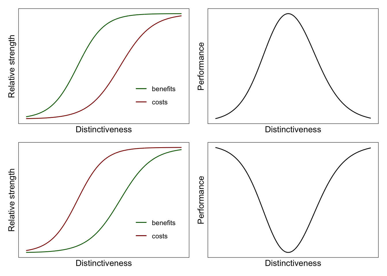

And if you want to, you can save it as a Latex file to import into your paper. The width and height are what I found to fit nicely in my Latex layout.

## create tikz file by specifying your path
tikz(file = "~/your/path/mech_plots.tex", width = 6.7, height = 3.4)

p1+p2+p3+p4+plot_layout(ncol = 2) ## gives you two columns-redundant in this case

dev.off()

If you want the OG Haans (2019) plots just specify the inverse-logit function and rerun the code. Note that I changed theme(legend.position) so that the labels do not overlap with the new plots.

f_logit <-function(b0,b1,b2,x) {
  exp((b0 +b1*x+b2*(x^2)))/(1+exp((b0 +b1*x+b2*(x^2))))
}

###generate s shapes for  u-shape parameters from Haans(2019)
df$competitive_gain <- f_logit(4,-12,0,df$distinctiveness)
df$legitimacy_loss <- f_logit(6,-10,0,df$distinctiveness)
df$inverted_u <-df$competitive_gain - df$legitimacy_loss
####generate s shapes for inverted u
df$competitive_gain_u <- f_logit(6,-10,0,df$distinctiveness)
df$legitimacy_loss_u <- f_logit(4,-12,0,df$distinctiveness)
df$u <-df$competitive_gain_u - df$legitimacy_loss_u

p1<- ggplot() +
  geom_line(data=df,aes(y = competitive_gain, x=distinctiveness, colour="benefits")) +
  geom_line(data=df,aes(y = legitimacy_loss, x=distinctiveness, colour="costs")) +
  scale_color_manual(name = "", values = c( "benefits" = "darkgreen", "costs" = "darkred"))+
  labs(y="Relative strength", x="Distinctiveness")+
  scale_y_continuous(breaks = NULL) +
  scale_x_continuous(breaks = NULL) +
  theme_bw()+ theme(legend.position = c(0.8,0.6))  

p2 <- ggplot() +
  geom_line(data=df,aes(y = inverted_u, x=distinctiveness))  +
  labs(y="Performance", x="Distinctiveness")+
  scale_y_continuous(breaks = NULL) +
  scale_x_continuous(breaks = NULL) +
  theme_bw()

p3 <- ggplot() +
  geom_line(data=df,aes(y = competitive_gain_u, x=distinctiveness, colour="benefits")) +
  geom_line(data=df,aes(y = legitimacy_loss_u, x=distinctiveness, colour="costs")) +
  scale_color_manual(name = "", values = c( "benefits" = "darkgreen", "costs" = "darkred"))+
  labs(y="Relative strength", x="Distinctiveness")+
  scale_y_continuous(breaks = NULL) +
  scale_x_continuous(breaks = NULL) +
  theme_bw()+ theme(legend.position = c(0.8,0.6))


p4 <- ggplot() +
  geom_line(data=df,aes(y = u, x=distinctiveness))  +  
  labs(y="Performance", x="Distinctiveness")+
  scale_y_continuous(breaks = NULL) +
  scale_x_continuous(breaks = NULL) +
  theme_bw()

###patchwork plots
p1+p2+p3+p4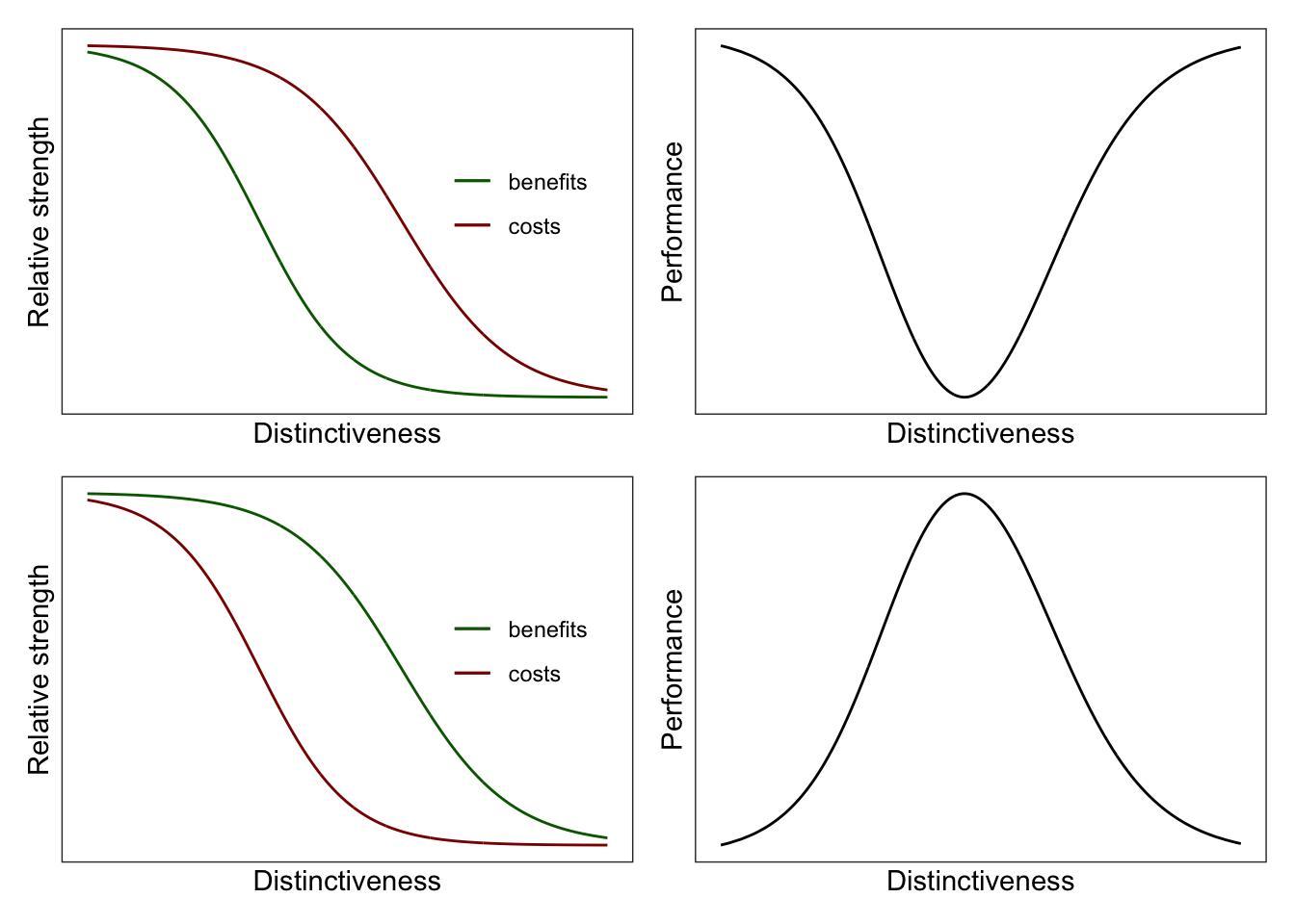

Enjoy!